Mis-Specified Weight Function
Adam Peterson
2018-11-03
WeightFunctions.RmdThe STAP framework requires a specified weight function, that desribes the rate at which the effect of the built environment feature either accumulates or decays across time or space respectively. This vignette explores and explains what happens when that weight function is mis-specified.
library(rstap)
library(dplyr)
library(tidyr)
library(ggplot2)set.seed(3421)
num_subj <- 5E2
num_bef <- 50
sub_df <- data_frame(x = runif(n = num_subj, min = 1, max = 2.0),
y = runif(n = num_subj, min = 1, max = 2.0),
class = "Subject")
bef_df <- data_frame(x = runif(n = num_bef, min = 0, max = 3.0),
y = runif(n = num_bef, min = 0, max = 3.0),
class = "BEF")
rbind(sub_df,bef_df) %>% ggplot(aes(x=x,y=y,color = class)) + geom_point() +
theme_bw() + ggtitle("Subject, BEF Spatial Arrangement")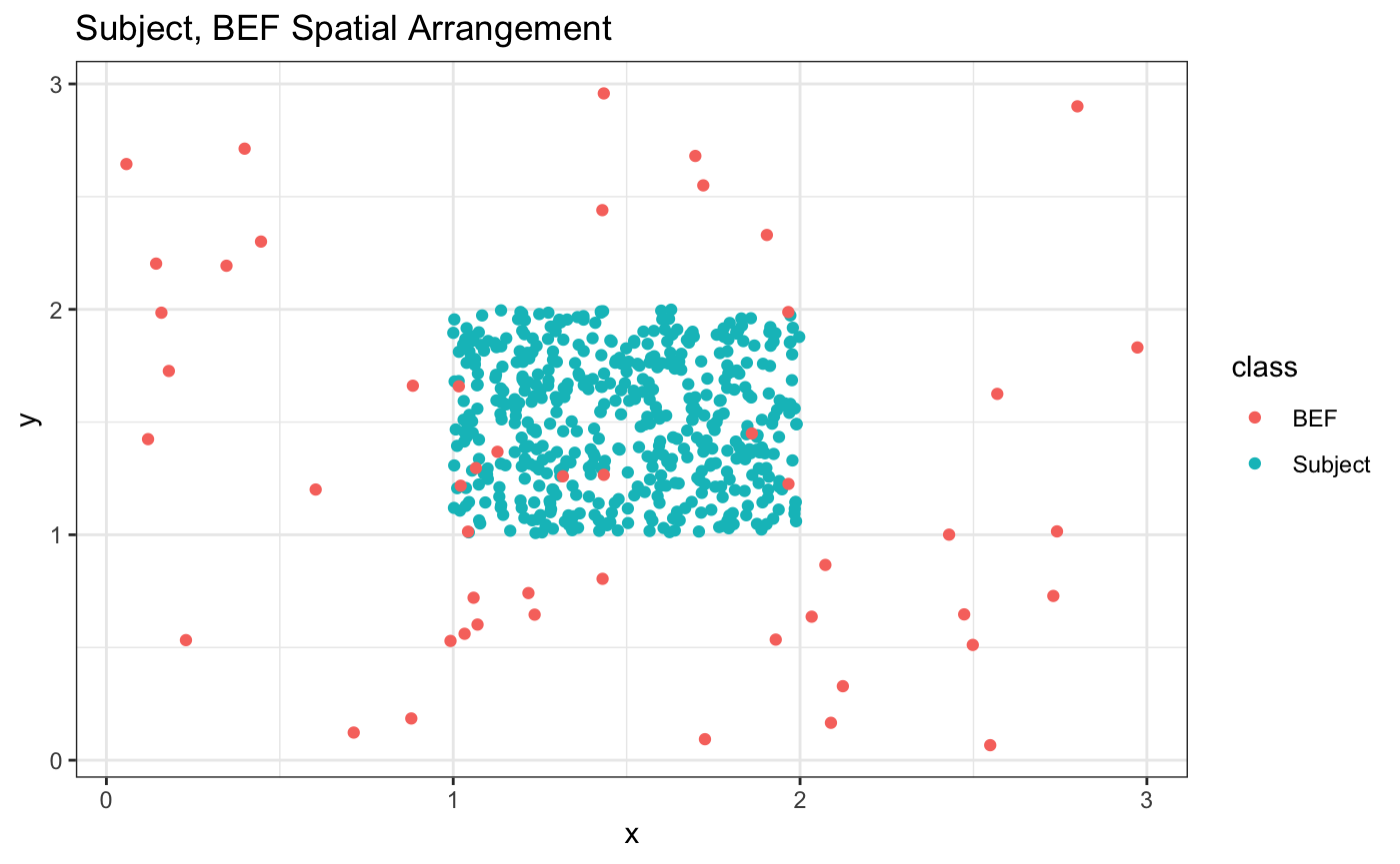
alpha <- 24
Z <- rbinom(n = num_subj,size = 1,prob = .5)
delta <- -.8
beta <- .92
theta_FF <- 2.00
theta_wei <- 4
sigma <- 1.3
true_pars <- c(alpha,delta,beta,theta_FF)
dists <- fields::rdist(as.matrix(sub_df[,c("x","y")]),
as.matrix(bef_df[,c("x","y")]))
unif_kernel <- function(x,theta) return( 1*(x<=theta) )
X_unif <- apply(dists,1,function(x) sum(unif_kernel(x,theta_FF)))
X_exp <- apply(dists,1,function(x) sum(exp(-x/theta_FF)))
X_wei <- apply(dists,1,function(x) sum(exp(-(x/theta_wei)^theta_wei)))
X_tilde <- as.matrix(scale(X_unif))
par(mfrow=c(1,2))
hist(dists)
hist(X_unif)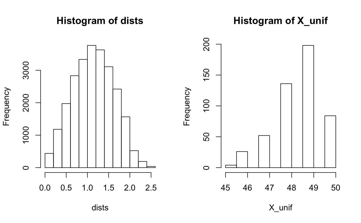
par(mfrow=c(1,2))
hist(X_exp)
hist(X_wei)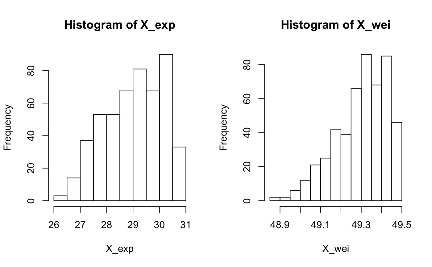
BMI_unif <- alpha + Z*delta + X_tilde*beta + rnorm(n = num_subj,mean = 0,sd = sigma)
BMI_exp <- alpha + Z*delta + scale(X_exp)*beta + rnorm(n = num_subj,mean = 0,sd = sigma)
BMI_wei <- alpha + Z*delta + scale(X_wei)*beta + rnorm(n = num_subj,mean = 0,sd = sigma)
par(mfrow=c(1,2))
d <- seq(from = 0, to = max(dists),by=0.01)
w_unif <- unif_kernel(d,theta_FF)
w_exp <- exp(-d/theta_FF)
theta_wei <- 4
w_wei <- exp(-(d/theta_wei)^theta_wei)
plot(d,pracma::erfc(d/theta_FF), type = 'l', main = "Cerf Decay")
plot(d,w_unif, type = 'l',main="Uniform Weight")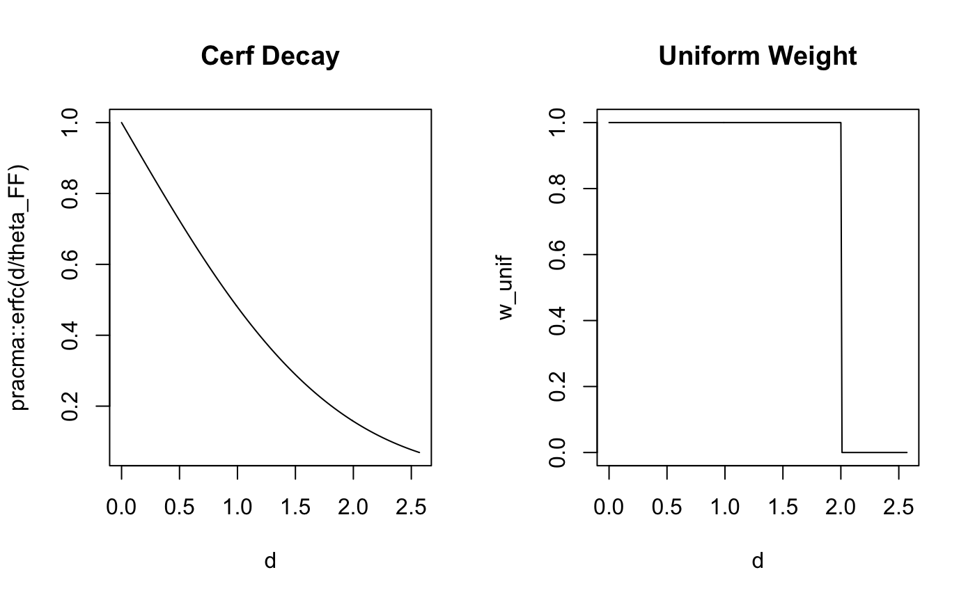
par(mfrow=c(1,2))
plot(d,w_exp, type = 'l',main = "Exponential decay")
plot(d,w_wei, type = 'l',main = "Weibull decay")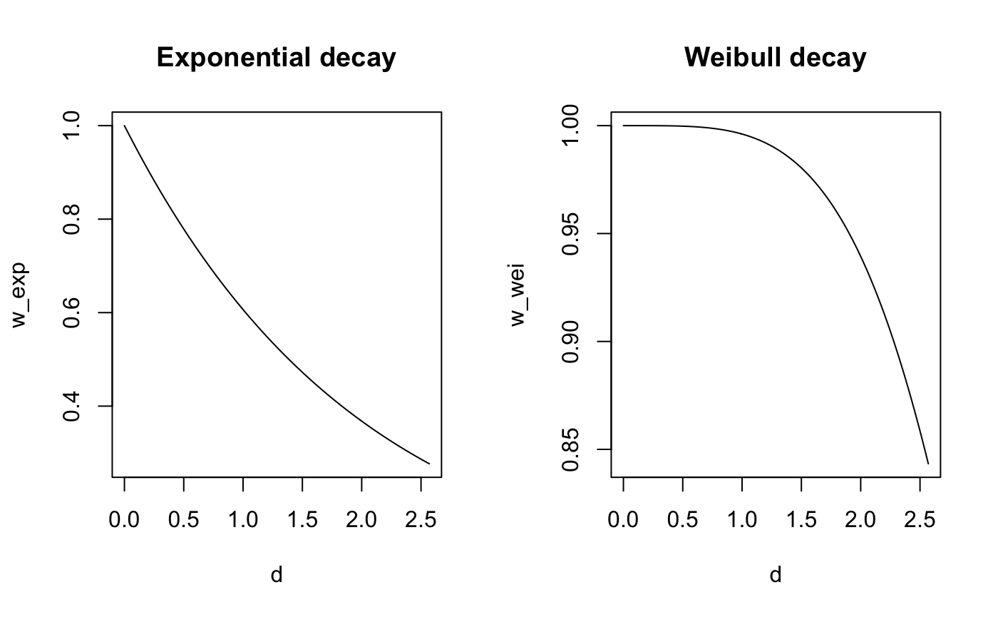
We’ll now model these data in the rstap framework, but since rstap’s estimation engine uses HMC, we can’t use a weight function that has a step-function. Instead we’ll use the usual complementary error function.
subj_df <- sub_df %>% mutate(BMI_exp = BMI_exp,
                             BMI_unif = BMI_unif,
                             BMI_we = BMI_wei,
                              sex = Z,
                              subj_id = 1:num_subj)

dist_df <- dists %>% as_data_frame() %>%
    mutate(subj_id = 1:nrow(subj_df)) %>%
    gather(contains("V"), key = 'BEF',value = 'Distance') %>%
    mutate(BEF = 'Fast_Food')

fit_unif <- stap_glm(formula = BMI_unif ~ sex + sap(Fast_Food),
                subject_data = subj_df,
                distance_data = dist_df,
                family = gaussian(link = 'identity'),
                subject_ID = 'subj_id',
                prior = normal(location = 0, scale = 5, autoscale = F),
                prior_intercept = normal(location = 26.2, scale = 5, autoscale = F),
                prior_stap = normal(location = 0, scale = 3, autoscale = F),
                prior_theta = log_normal(location = 1, scale = 1),
                prior_aux = cauchy(location = 0,scale = 5),
max_distance = max(dists), chains = 2, cores = 2)summary(fit_unif,waic=T)
#>
#> Model Info:
#>
#> function: stap_glm
#> family: gaussian [identity]
#> formula: BMI_unif ~ sex + sap(Fast_Food)
#> priors: see help('prior_summary')
#> sample: 2000 (posterior sample size)
#> observations: 500
#> Spatial Predictors: 1
#> WAIC: 1832.4
#>
#> Estimates:
#> mean sd 2.5% 25% 50% 75% 97.5%
#> (Intercept) -0.7 25.6 -65.5 -6.3 6.8 14.2 21.6
#> sex -0.7 0.1 -0.9 -0.8 -0.7 -0.6 -0.4
#> Fast_Food 0.6 0.5 0.1 0.3 0.4 0.7 1.9
#> Fast_Food_spatial_scale 10.0 8.4 2.6 5.2 7.6 11.9 32.5
#> sigma 1.5 0.0 1.4 1.5 1.5 1.5 1.6
#> mean_PPD 23.6 0.1 23.4 23.5 23.6 23.6 23.8
#> log-posterior -925.4 1.8 -929.9 -926.2 -925.0 -924.1 -923.1
#>
#> Diagnostics:
#> mcse Rhat n_eff
#> (Intercept) 0.8 1.0 1049
#> sex 0.0 1.0 2304
#> Fast_Food 0.0 1.0 1045
#> Fast_Food_spatial_scale 0.3 1.0 1002
#> sigma 0.0 1.0 1682
#> mean_PPD 0.0 1.0 2010
#> log-posterior 0.1 1.0 678
#>
#> For each parameter, mcse is Monte Carlo standard error, n_eff is a crude measure of effective sample size, and Rhat is the potential scale reduction factor on split chains (at convergence Rhat=1).as.matrix(fit_unif) %>% as_data_frame() %>%
mutate(prior = rlnorm(n=n(),meanlog = 1,sdlog = 1)) %>%
gather(everything(),key ='parameter',value = 'sample') %>%
filter(parameter%in%c("Fast_Food_spatial_scale","prior")) %>%
ggplot(aes(x=sample,color=parameter)) + geom_density() + theme_bw() +
ggtitle("Prior vs. Posterior Comparison")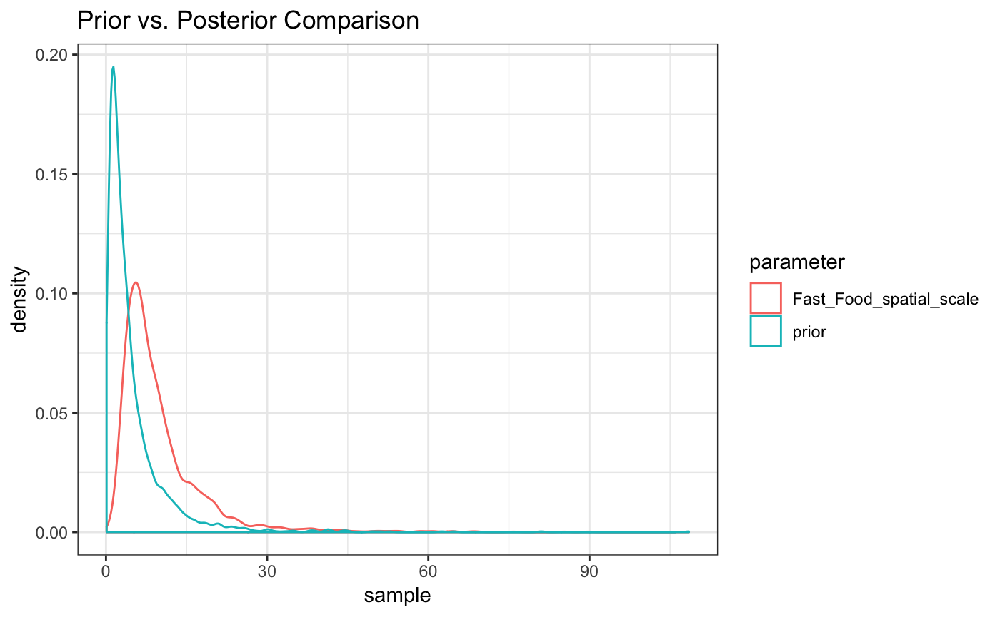
d <- seq(from = 0, to = max(dists), by = 0.01)
cerf_w <- pracma::erfc(d/coef(fit_unif)[4])
unif_w <- unif_kernel(d,theta_FF)
par(mfrow=c(1,2))
plot(d,cerf_w, main = "Cerf Weight", type='l')
points(d,pracma::erfc(d/posterior_interval(fit_unif,regex_pars = 'scale')[1]),col='red', type = 'l',lty=2)
points(d,pracma::erfc(d/posterior_interval(fit_unif,regex_pars = 'scale')[2]),col='red', type = 'l',lty=2)
plot(d,unif_w, main = "Unif Weight", type='l')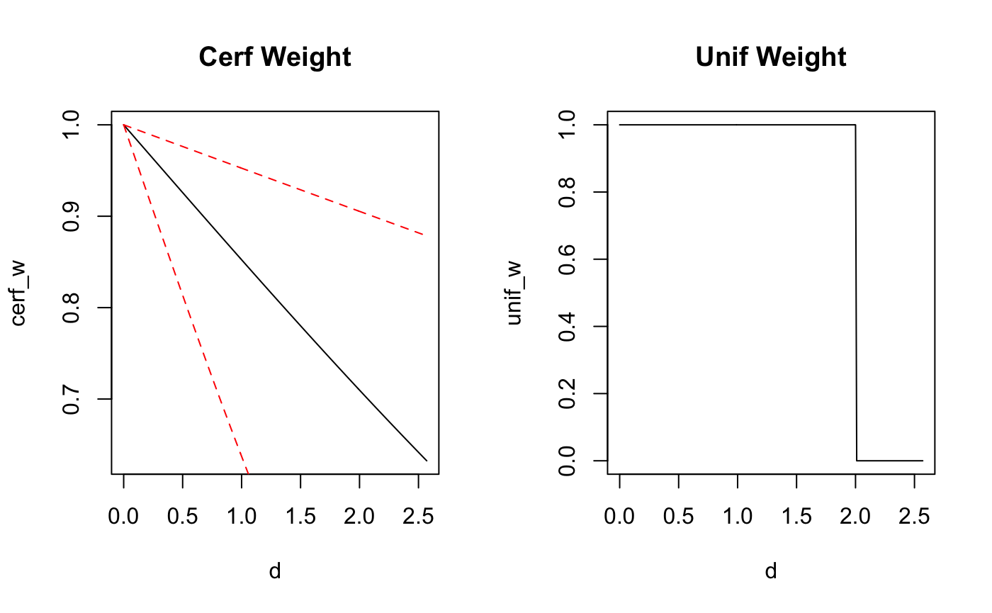
For a different, more closely related weight function, the discrepancy might not be as bad.
fit_exp <- stap_glm(formula = BMI_exp ~ sex + sap(Fast_Food),
                subject_data = subj_df,
                distance_data = dist_df,
                family = gaussian(link = 'identity'),
                subject_ID = 'subj_id',
                prior = normal(location = 0, scale = 5, autoscale = F),
                prior_intercept = normal(location = 26.2, scale = 5, autoscale = F),
                prior_stap = normal(location = 0, scale = 3, autoscale = F),
                prior_theta = log_normal(location = 1, scale = 1),
                prior_aux = cauchy(location = 0,scale = 5),
max_distance = max(dists), chains = 2, cores = 2)summary(fit_exp,waic=T)
#>
#> Model Info:
#>
#> function: stap_glm
#> family: gaussian [identity]
#> formula: BMI_exp ~ sex + sap(Fast_Food)
#> priors: see help('prior_summary')
#> sample: 2000 (posterior sample size)
#> observations: 500
#> Spatial Predictors: 1
#> WAIC: 1646
#>
#> Estimates:
#> mean sd 2.5% 25% 50% 75% 97.5%
#> (Intercept) -3.1 35.0 -98.3 -5.3 7.9 13.7 18.4
#> sex -0.7 0.1 -0.9 -0.8 -0.7 -0.6 -0.5
#> Fast_Food 0.8 0.7 0.4 0.5 0.6 0.8 2.7
#> Fast_Food_spatial_scale 4.0 4.0 1.3 2.0 2.7 4.3 15.2
#> sigma 1.3 0.0 1.2 1.2 1.2 1.3 1.3
#> mean_PPD 23.6 0.1 23.4 23.5 23.6 23.6 23.8
#> log-posterior -829.8 1.6 -833.7 -830.7 -829.5 -828.6 -827.6
#>
#> Diagnostics:
#> mcse Rhat n_eff
#> (Intercept) 1.1 1.0 1050
#> sex 0.0 1.0 2139
#> Fast_Food 0.0 1.0 1047
#> Fast_Food_spatial_scale 0.1 1.0 1036
#> sigma 0.0 1.0 1883
#> mean_PPD 0.0 1.0 2111
#> log-posterior 0.1 1.0 831
#>
#> For each parameter, mcse is Monte Carlo standard error, n_eff is a crude measure of effective sample size, and Rhat is the potential scale reduction factor on split chains (at convergence Rhat=1).as.matrix(fit_exp) %>% as_data_frame() %>%
mutate(prior = rlnorm(n=n(),meanlog = 1,sdlog = 1)) %>%
gather(everything(),key ='parameter',value = 'sample') %>%
filter(parameter%in%c("Fast_Food_spatial_scale","prior")) %>%
ggplot(aes(x=sample,color=parameter)) + geom_density() + theme_bw() +
ggtitle("Prior vs. Posterior Comparison")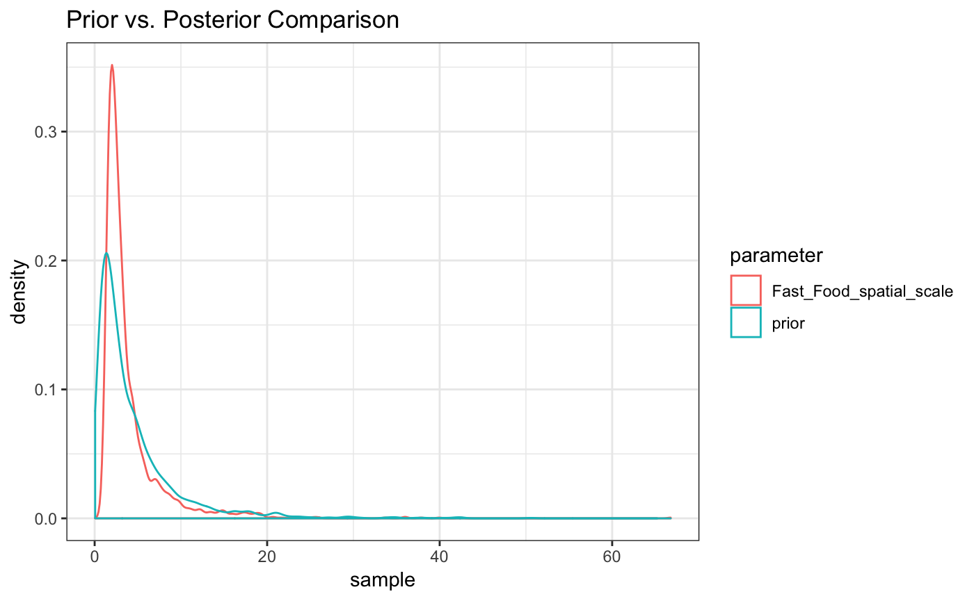
d <- seq(from = 0, to = max(dists), by = 0.01)
cerf_w <- pracma::erfc(d/coef(fit_exp)[4])
exp_w <- exp(-d/theta_FF)
plot(d,cerf_w, main = "Cerf Weight", type='l')
points(d,pracma::erfc(d/posterior_interval(fit_exp,regex_pars = 'scale')[1]),col='red', type = 'l', lty = 2)
points(d,pracma::erfc(d/posterior_interval(fit_exp,regex_pars = 'scale')[2]),col='red', type = 'l', lty = 2)
points(d,exp_w, main = "Exponential Weight", type='l',col='blue',lty=3, lwd = 2)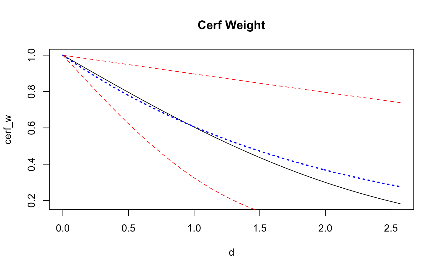
Using the exact spatial temporal predictor now…
fit_exp2 <- stap_glm(formula = BMI_exp ~ sex + sap(Fast_Food,exp),
subject_data = subj_df,
distance_data = dist_df,
family = gaussian(link = 'identity'),
subject_ID = 'subj_id',
prior = normal(location = 0, scale = 5, autoscale = F),
prior_intercept = normal(location = 26.2, scale = 5, autoscale = F),
prior_stap = normal(location = 0, scale = 3, autoscale = F),
prior_theta = log_normal(location = 1, scale = 1),
prior_aux = cauchy(location = 0,scale = 5),
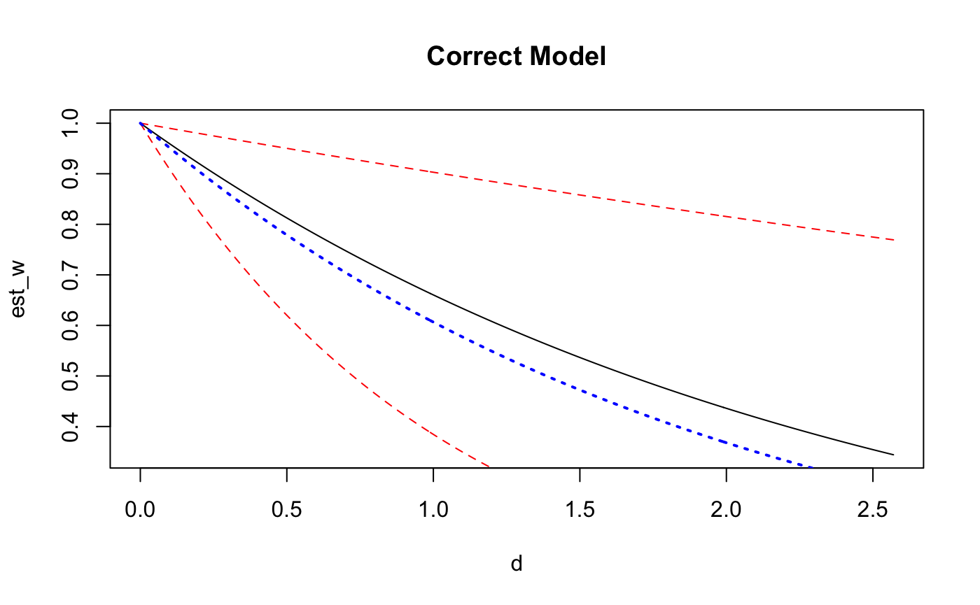
max_distance = max(dists), chains = 2, cores = 2)Examining the WAIC we see that the correct model has - ever so slightly - better fit than the error function approximation. This is likely because the two functiosn are so closely related. Still there may be other functions for which one serves as a better approximation than the other - WAIC can provide some guide to this.
summary(fit_exp2,waic=T)
#>
#> Model Info:
#>
#>  function:     stap_glm
#>  family:       gaussian [identity]
#>  formula:      BMI_exp ~ sex + sap(Fast_Food, exp)
#>  priors:       see help('prior_summary')
#>  sample:       2000 (posterior sample size)
#>  observations: 500
#>  Spatial Predictors:   1
#>  WAIC: 1645.3
#>
#> Estimates:
#>                           mean   sd     2.5%   25%    50%    75%    97.5%
#> (Intercept)              -10.8   36.7 -110.4  -14.9    0.6    8.8   16.0
#> sex                       -0.7    0.1   -0.9   -0.8   -0.7   -0.6   -0.5
#> Fast_Food                  1.0    0.7    0.5    0.6    0.7    1.0    2.9
#> Fast_Food_spatial_scale    3.6    3.6    0.9    1.6    2.4    4.0   13.6
#> sigma                      1.2    0.0    1.2    1.2    1.2    1.3    1.3
#> mean_PPD                  23.6    0.1   23.4   23.5   23.6   23.7   23.8
#> log-posterior           -829.6    1.6 -833.6 -830.4 -829.3 -828.4 -827.4
#>
#> Diagnostics:
#>                         mcse Rhat n_eff
#> (Intercept)             1.1  1.0  1042
#> sex                     0.0  1.0  2653
#> Fast_Food               0.0  1.0  1036
#> Fast_Food_spatial_scale 0.1  1.0   991
#> sigma                   0.0  1.0  2165
#> mean_PPD                0.0  1.0  1870
#> log-posterior           0.1  1.0   775
#>
#> For each parameter, mcse is Monte Carlo standard error, n_eff is a crude measure of effective sample size, and Rhat is the potential scale reduction factor on split chains (at convergence Rhat=1).as.matrix(fit_exp2) %>% as_data_frame() %>%
mutate(prior = rlnorm(n=n(),meanlog = 1,sdlog = 1)) %>%
gather(everything(),key ='parameter',value = 'sample') %>%
filter(parameter%in%c("Fast_Food_spatial_scale","prior")) %>%
ggplot(aes(x=sample,color=parameter)) + geom_density() + theme_bw() +
ggtitle("Prior vs. Posterior Comparison")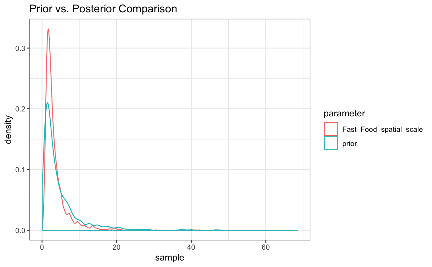
d <- seq(from = 0, to = max(dists), by = 0.01)
est_w <- exp(-d/coef(fit_exp2)[4])
exp_w <- exp(-(d/theta_FF))
plot(d,est_w, main = "Correct Model", type='l')
points(d,exp(-d/posterior_interval(fit_exp2,regex_pars = 'scale')[1]),col='red', type = 'l', lty = 2)
points(d,exp(-d/posterior_interval(fit_exp2,regex_pars = 'scale')[2]),col='red', type = 'l', lty = 2)
points(d,exp_w, type='l',col='blue',lty=3, lwd = 2)